
 Shibuya
jupyter-sphinx#
Jupyter-sphinx is a Sphinx extension that executes embedded code in a Jupyter kernel, and embeds outputs of that code in the document.
Documentation: https://jupyter-sphinx.readthedocs.io/
Source Code: https://github.com/jupyter/jupyter-sphinx
Install#
pip install jupyter-sphinx
Then, add the extension to your conf.py:
extensions = [
    # ...
    "jupyter_sphinx",
]
If you encounter this error:
Unable to find kernel (exception: No such kernel named python3)
Try to install ipykernel:
pip install ipykernel
Usage#
You can use the jupyter-execute directive to embed code into the document:
.. jupyter-execute::

  name = 'world'
  print('hello ' + name + '!')
The above is rendered as follows:
name = 'world'
print('hello ' + name + '!')
hello world!
Note that the code produces output (printing the string ‘hello world!’), and the output is rendered directly after the code snippet.
Because all code cells in a document are run in the same kernel, cells later in the document can use variables and functions defined in cells earlier in the document:
a = 1
print('first cell: a = {}'.format(a))
first cell: a = 1
a += 1
print('second cell: a = {}'.format(a))
second cell: a = 2
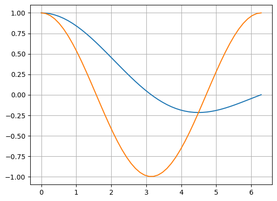
Because jupyter-sphinx uses the machinery of nbconvert, it is capable of rendering any rich output, for example plots:
import numpy as np
from matplotlib import pyplot
%matplotlib inline

x = np.linspace(1E-3, 2 * np.pi)

pyplot.plot(x, np.sin(x) / x)
pyplot.plot(x, np.cos(x))
pyplot.grid()
LaTeX output:
from IPython.display import Latex
Latex(r'\int_{-\infty}^\infty e^{-x²}dx = \sqrt{\pi}')
or even full-blown javascript widgets:
import ipywidgets as w
from IPython.display import display

a = w.IntSlider()
b = w.IntText()
w.jslink((a, 'value'), (b, 'value'))
display(a, b)
It is also possible to include code from a regular file by passing the filename as argument
to jupyter-execute:
.. jupyter-execute:: some_code.py
jupyter-execute may also be used in docstrings within your Python code, and will be executed
when they are included with Sphinx autodoc.
Directive options#
You may choose to hide the code of a cell, but keep its output visible using :hide-code::
.. jupyter-execute::
    :hide-code:

    print('this code is invisible')
produces:
print('this code is invisible')
this code is invisible
this option is particularly useful if you want to embed correctness checks in building your documentation:
.. jupyter-execute::
    :hide-code:

    assert everything_works, "There's a bug somewhere"
This way even though the code won’t make it into the documentation, the build will fail if running the code fails.
Similarly, outputs are hidden with :hide-output::
.. jupyter-execute::
    :hide-output:

    print('this output is invisible')
produces:
print('this output is invisible')
You may also display the code below the output with :code-below::
.. jupyter-execute::
    :code-below:

    print('this code is below the output')
produces:
this code is below the output
print('this code is below the output')
You may also add line numbers to the source code with :linenos::
.. jupyter-execute::
   :linenos:

   print('A')
   print('B')
   print('C')
produces:
1print('A')
2print('B')
3print('C')
A
B
C
To add line numbers from a specific line to the source code, use the
lineno-start directive:
.. jupyter-execute::
   :lineno-start: 7

   print('A')
   print('B')
   print('C')
produces:
7print('A')
8print('B')
9print('C')
A
B
C
You may also emphasize particular lines in the source code with :emphasize-lines::
.. jupyter-execute::
    :emphasize-lines: 2,5-6

    d = {
        'a': 1,
        'b': 2,
        'c': 3,
        'd': 4,
        'e': 5,
    }
produces:
2d = {
3    'a': 1,
4    'b': 2,
5    'c': 3,
6    'd': 4,
7    'e': 5,
8}
Controlling exceptions#
The default behaviour when jupyter-sphinx encounters an error in the embedded code is just to
stop execution of the document and display a stack trace. However, there are many cases where it may be
illustrative for execution to continue and for a stack trace to be shown as output of the cell. This
behaviour can be enabled by using the raises option:
.. jupyter-execute::
    :raises:

    1 / 0
produces:
1 / 0
---------------------------------------------------------------------------
ZeroDivisionError                         Traceback (most recent call last)
Cell In[13], line 1
----> 1 1 / 0

ZeroDivisionError: division by zero
Note that when given no arguments, raises will catch all errors. It is also possible to give raises
a list of error types; if an error is raised that is not in the list then execution stops as usual:
.. jupyter-execute::
    :raises: KeyError, ValueError

    a = {'hello': 'world!'}
    a['jello']
produces:
a = {'hello': 'world!'}
a['jello']
---------------------------------------------------------------------------
KeyError                                  Traceback (most recent call last)
Cell In[14], line 2
      1 a = {'hello': 'world!'}
----> 2 a['jello']

KeyError: 'jello'
Additionally, any output sent to the stderr stream of a cell will result in jupyter-sphinx
producing a warning. This behaviour can be suppressed (and the stderr stream printed as regular
output) by providing the stderr option:
.. jupyter-execute::
    :stderr:

    import sys

    print("hello, world!", file=sys.stderr)
produces:
import sys

print("hello, world!", file=sys.stderr)
hello, world!
Manually forming Jupyter cells#
When showing code samples that are computationally expensive, access restricted resources, or have non-deterministic output, it can be preferable to not have them run every time you build. You can simply embed input code without executing it using the jupyter-input directive expected output with jupyter-output:
.. jupyter-input::
    :linenos:

    import time

    def slow_print(str):
        time.sleep(4000)    # Simulate an expensive process
        print(str)

    slow_print("hello, world!")

.. jupyter-output::

    hello, world!
produces:
1import time
2
3def slow_print(str):
4    time.sleep(4000)    # Simulate an expensive process
5    print(str)
6
7slow_print("hello, world!")
hello, world!